Convex Sets in High Dimensions

by Tomasz Tkocz

This note briefly surveys several results, classical by now, which shaped high-dimensional convex geometry and describes its major open problems. We start with a closer look at Euclidean balls and then try to make a point that “in high-dimensions, all convex sets, despite their rich structure, behave a bit like Euclidean balls”.

A set of points \(A\) in \(R^n\) is called convex if along with every two points \(a_1, a_2\) in \(A\), the whole segment \([a_1,a_2]\) joining \(a_1\) and \(a_2\) is contained in the set \(A\). For example balls and ellipsoids, or cubes and parallelopipeds are convex, whereas annuli are not. How is volume distributed in a convex set? Say, we have a convex set of volume \(1\). Where is most of its volume concentrated?

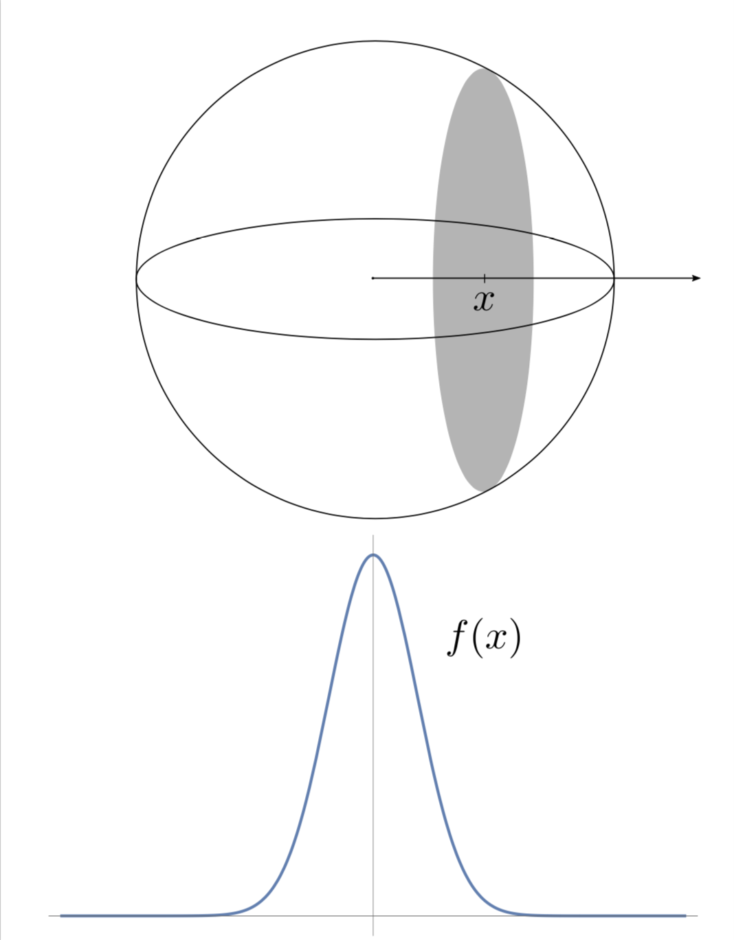
Consider the example of a centered Euclidean ball \(B = \{x \in R^n, \ x_1^2+\ldots+x_n^2 \leq r^2\}\). Choose its radius \(r\) such that it has unit volume, \(r = v_n^{-1/n}\), where \(v_n\) is the volume of the $n$-dimensional ball with radius \(1\). Thus, \(r = \frac{1}{\sqrt{\pi}}\Gamma(1+\frac{n}{2})^{1/n}\), which is approximately \(\sqrt{\frac{n}{2\pi e}}\) for large \(n\). For \(x \in R\), let \(f(x)\) be the \((n-1)\)-dimensional volume of the cross-section of \(B\) with a hyperplane perpendicular to the \(0x_1\) axis passing through \((x,0,\ldots,0)\). Plainly,
\[
\int_{-\infty}^{\infty} f(x) dd x = vol(B) = 1.
\]

The function \(f\) is the probability density of the volume distribution of the ball \(B\) in the direction of the vector \((1,0,\ldots,0)\). What is this distribution like? That cross-section is again a ball, whose radius is \(\sqrt{r^2-x^2}\) (Pythagoras’ theorem). Therefore,
\[
f(x) = \sqrt{r^2-x^2}^{n-1}v_{n-1} = \left(1 – \frac{x^2}{r^2}\right)^{\frac{n-1}{2}}r^{n-1}v_{n-1}
\]
We check that \(r^{n-1}v_{n-1} \approx \sqrt{e}\) for large \(n\) and when \(x\) is much smaller than \(r\), we can write \(1-(x/r)^2 \approx e^{-(x/r)^2}\) and thus conclude that, approximately,
\[
f(x) \approx \sqrt{e}e^{-\pi e x^2}.
\]

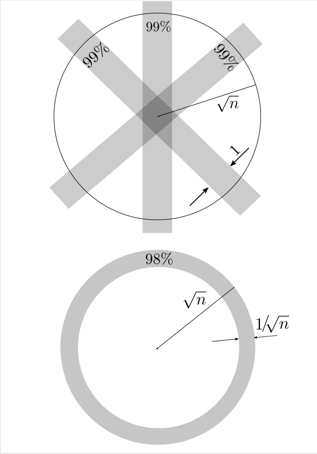
This means that \(f\), the volume distribution in the ball \(B\) is roughly Gaussian with variance \(\sigma\) of constant order (\(\sigma = \frac{1}{2\pi e}\))! So, where is the volume concentrated? By the \(3\sigma\)-rule, \(\int_{-3\sigma}^{3\sigma} f(x) dd x > 0.99\), so more than \(99\%\) volume of \(B\) is within a symmetric slab \(\{x \in R^n, \ |x_1| \leq 3\sigma\}\) of width \(6\sigma\). In high dimension \(n\), this width of constant order becomes tiny tiny in comparison with the radius \(r\) of \(B\), which is of the order \(\sqrt{n}\). To challenge our high dimensional intuitions more, remark that the choice of the axis \(0x_1\) was arbitrary and by symmetry the above remains true for any other direction, so \(99\%\) volume of \(B\) is within any symmetric slab of width \(6\sigma\).

Let us have a look at how much volume there is near the surface of \(B\), say in an annulus of the inner radius \(r – 1/\sqrt{n}\) and the outer radius \(r\), for some constant \(C\). Plainly, this volume equals
\[
1 – \left(\frac{r-1/\sqrt{n}}{r}\right)^n = 1 – \left(1 – \frac{1}{r\sqrt{n}}\right)^n \approx 1 – e^{-\frac{n}{r\sqrt{n}}} \approx 1 – e^{-\sqrt{2\pi e}} \approx 0.98.
\]
This means that on one hand, almost all the volume of \(B\) is within any symmetric slab of constant width (hence also in the intersection of many of those), and on the other hand, almost all the volume of \(B\) is concentrated near its surface (in an annulus of width $1/\sqrt{n}$).

Asymptotic convex geometry is concerned with quantifying such high dimensional phenomena for arbitrary convex sets. One of the major breakthroughs was Klartag’s central limit theorem which guarantees that the same phenomenon which we observed above for the ball holds for an arbitrary convex set (properly normalised): the distribution of volume (function \(f\)) is Gaussian along most of directions. It was explained by Antilla, Ball and Peresinaki that such a central limit behavior comes from the volume being concentrated in a thin annulus, as readily observed above for the Euclidean ball. Klartag established this type of estimates, called thin-shell bounds, for an arbitrary convex set \(K\) in \(R^n\), showing that there are sequences \(\delta_n, \varepsilon_n \to 0\) as \(n \to \infty\) such that
\[
\frac{1}{vol(K)}vol\left\{x \in R^n, \ 1-\varepsilon_n \leq \frac{|x|}{\sqrt{n}} \leq 1+\varepsilon_n \right\} \geq 1 – \delta_n,
\]
provided that \(K\) is properly normalised (its inertia matrix being the identity).

Historically, asymptotic convex geometry grew out of Dvoretzky’s theorem, which says that \(n\)-dimensional symmetric convex sets admit sections with roughly \(\log n\)-dimensional subspaces which are almost Euclidean balls. Interestingly, such Euclidean subspaces are not easy to find constructively, however, Milman’s probabilistic proof of Dvoretzky’s theorem shows that most subspaces yield Euclidean sections.

Of course, many problems remain unsolved. A central one, the slicing problem posed by Bourgain, asks whether there is a universal constant \(c\) such that for every dimension \(n\), every \(n\)-dimensional convex set with volume \(1\) admits a codimension \(1\) section through its barycentre of volume at least \(c\). (Currently the best dimension dependent bound on \(c\) is of the order \(n^{-1/4}\)).

The slicing problem is equivalent to many other natural questions in convex geometry and beyond. For example, the Busemann-Petty problem asked the following: if symmetric convex sets \(K\) and \(L\) in \(R^n\) satisfy \(vol(K \cap H) \leq vol(L \cap H)\) for every codimension \(1\) subspace, does it follow that \(vol(K) \leq vol(L)\)? After a bit of dramatic history, the problem was solved completely and the answer is affirmative if and only if \(n \leq 4\) (for \(n \geq 10\), a cube and a ball give a counter-example). Proving that \(vol(K) \leq C vol(L)\) for a universal constant \(C\) would also solve the slicing problem in the affirmative. Another example concerns information theory: the slicing problem is equivalent to showing that the relative entropy per coordinate of every uniform distribution on a convex set does not exceed a universal constant. The links with information theory were also fruitful to establish unexpected connections between the slicing problem and other major open problems, such as the Kannan-Lovász-Simonovits conjecture (which in turn has its roots in devising efficient algorithms for computing volumes of convex sets).

Further reading
Giannopoulos, A., Milman, V., Asymptotic
convex geometry: short overview.
Different Faces of Geometry, 87-162, Int. Math. Ser. (N. Y.), 3, 2004.